How to Use Excel Like a Pro: 18 Easy Excel Tips, Tricks, & Shortcuts

Veritably, Excel appears to be like too actual to be fair. All I occupy to enact is enter a formulation, and highest powerful the leisure I would ever must enact manually is also carried out automatically. Want to merge two sheets with identical data? Excel can enact it. Want to enact straightforward math? Excel can enact it. Want to mix info in more than one cells? Excel can enact it.

The handiest downside is that it will also be sophisticated to make use of for inexperienced persons. Whereas inputting the info manually is easy, it in total is a nightmare to learn your entire system and shortcuts you’d like to master the tool. Plus, even whenever you use the system precisely, there’s continuously a chance you’ll speed into error messages. Merely attach, Excel is also extraordinarily hard to make use of.

Not to peril. In this put up, I’ll mosey over the highest attainable methods, tricks, and shortcuts you must possibly perhaps possibly possibly also use appropriate now to prefer your Excel sport to the next level. No developed Excel data required.

What’s Excel?

Microsoft Excel is a spreadsheet machine that marketers, accountants, data analysts, and diversified professionals use to store, manage, and observe data devices. It’s segment of the Microsoft Plan of enterprise suite of products. Probably decisions include Google Sheets and Numbers. Gain more Excel decisions here.

To jumpstart your Excel education, take a look at up on a video beneath on easy methods on how to make use of Excel for inexperienced persons.

Excel is essentially used for creating financial documents due to its tough computational powers. You’ll continually obtain the machine in accounting offices and teams because it enables accountants to automatically gaze sums, averages, and totals. With Excel, they’ll without considerations make sense of their industry’ data.

Whereas Excel is essentially identified as an accounting tool, professionals in any area can use its parts and system — in particular marketers — because it will also be used for monitoring any form of data. It will get rid of the must exhaust hours and hours counting cells or copying and pasting performance numbers. Excel in most cases has a shortcut or hastily fix that accelerates the technique.

Not certain the manner to genuinely use Excel in your crew? Here’s a record of documents you must possibly perhaps possibly possibly also occupy:

• Earnings Statements: You have to possibly possibly also use an Excel spreadsheet to computer screen an organization’s sales activity and financial effectively being.
• Steadiness Sheets: Steadiness sheets are amongst basically the most neatly-liked kinds of documents you must possibly perhaps possibly possibly also occupy with Excel. It enables you to earn a holistic observe of an organization’s financial standing.
• Calendar: You have to possibly possibly also without considerations occupy a spreadsheet month-to-month calendar to computer screen events or diversified date-composed info.

Here are some documents you must possibly perhaps possibly possibly also occupy particularly for marketers.

• Marketing Budgets: Excel is a strong budget-retaining tool. You have to possibly possibly also occupy and observe marketing budgets, to boot to exhaust, the use of Excel. For fogeys that don’t would love to occupy a doc from scratch, download our marketing budget templates for free.
• Marketing Experiences: For fogeys that don’t use a marketing tool equivalent to Marketing Hub, you must possibly perhaps possibly possibly also obtain your self wanting a dashboard with all of your experiences. Excel is a shining tool to occupy marketing experiences. Download free Excel marketing reporting templates here.
• Editorial Calendars: You have to possibly possibly also occupy editorial calendars in Excel. The tab layout makes it extraordinarily easy to computer screen your speak creation efforts for custom time ranges. Download a free editorial speak calendar template here.
• Traffic and Leads Calculator: Because of its tough computational powers, Excel is a shining tool to occupy all kinds of calculators — along with one for monitoring leads and visitors. Click here to download a free premade calculator.

Here is handiest a minute sampling of the categories of promoting and industry documents you must possibly perhaps possibly possibly also occupy in Excel. We’ve created an intensive record of Excel templates you must possibly perhaps possibly possibly also use appropriate now for marketing, invoicing, project management, budgeting, and more.

You have to possibly possibly also furthermore download Excel templates beneath for all of your marketing needs. 

After you download the templates, it’s time to birth up the use of the machine. Let’s veil the fundamentals first.

Excel Basics

For fogeys that’re criminal initiating out with Excel, there are just a few standard instructions that we advocate you become mindful of. These are things like:

• Creating a brand new spreadsheet from scratch.
• Executing standard computations like adding, subtracting, multiplying, and dividing.
• Writing and formatting column text and titles.
• The use of Excel’s auto-occupy parts.
• Including or deleting single columns, rows, and spreadsheets. Below, we’ll earn into easy methods on how so as to add things like more than one columns and rows.
• Holding column and row titles visible as you scroll past them in a spreadsheet, so that what data you’re filling as you switch additional down the doc.

For a deep dive on these basics, take a look at up on our total Microsoft Excel handbook.

In the spirit of working more efficiently and heading off behind, manual work, listed below are just a few Excel system and capabilities you’ll must know.

Excel Formulas

It’s easy to earn overwhelmed by the shining selection of Excel system that you must possibly perhaps possibly possibly also use to make sense out of your data. For fogeys that’re criminal getting started the use of Excel, you must possibly perhaps possibly possibly also count on the next system to attain some advanced capabilities — without adding to the complexity of your learning path.

• Equal signal: Earlier than creating any formulation, you’ll must write an equal signal (=) in the cell where you’d like to occupy the consequence to appear.
• Addition: To add the values of two or more cells, use the + signal. Example: =C5+D3.
• Subtraction: To subtract the values of two or more cells, use the – signal. Example: =C5-D3.
• Multiplication: To multiply the values of two or more cells, use the * signal. Example: =C5*D3.
• Division: To divide the values of two or more cells, use the / signal. Example: =C5/D3.

Placing all of these together, you must possibly perhaps possibly possibly also occupy a formulation that adds, subtracts, multiplies, and divides all in a single cell. Example: =(C5-D3)/((A5+B6)*3).

For more advanced system, you’ll must make use of parentheses all the arrangement in which by the expressions to dwell a ways from accidentally the use of the PEMDAS mutter of operations. Aid in thoughts that you must possibly perhaps possibly possibly also use horrid numbers in your system.

Excel Functions

Excel capabilities automate a few of the tasks you would possibly want to utilize in a common formulation. Let’s divulge, as any other of the use of the + signal so as to add up a large range of cells, you’d use the SUM feature. Let’s gape at just a few more capabilities that will attend automate calculations and tasks.

• SUM: The SUM feature automatically adds up a large range of cells or numbers. To entire a sum, you can input the initiating cell and the highest attainable cell with a colon in between. Here’s what that seems as if: SUM(Cell1:Cell2). Example: =SUM(C5:C30).
• AVERAGE: The AVERAGE feature averages out the values of a big range of cells. The syntax is the identical because the SUM feature: AVERAGE(Cell1:Cell2). Example: =AVERAGE(C5:C30).
• IF: The IF feature enables you to return values essentially based entirely on a logical take a look at. The syntax is as follows: IF(logical_test, value_if_true, [value_if_false]). Example: =IF(A2>B2,”Over Budget”,”OK”).
• VLOOKUP: The VLOOKUP feature helps you gape the leisure in your sheet’s rows. The syntax is: VLOOKUP(look up worth, desk array, column number, Approximate match (TRUE) or Accurate match (FALSE)). Example: =VLOOKUP([@Attorney],tbl_Attorneys,4,FALSE).
• INDEX: The INDEX feature returns a worth from within a form. The syntax is as follows: INDEX(array, row_num, [column_num]).
• MATCH: The MATCH feature seems for a certain merchandise in a large range of cells and returns the predicament of that merchandise. It’s going to also be used in tandem with the INDEX feature. The syntax is: MATCH(lookup_value, lookup_array, [match_type]).
• COUNTIF: The COUNTIF feature returns the sequence of cells that meet a certain requirements or occupy a certain worth. The syntax is: COUNTIF(fluctuate, requirements). Example: =COUNTIF(A2:A5,”London”).

Okay, ready to earn into the nitty-gritty? Let’s earn to it. (And to your entire Harry Potter followers available in the market … you’re welcome upfront.)

Demonstrate: The GIFs and visuals are from a previous model of Excel. When acceptable, the replica has been up previously to create instruction for customers of both more moderen and older Excel variations.

1. Use Pivot tables to stare and make sense of data.

Pivot tables are used to reorganize data in a spreadsheet. They is no longer any longer going to commerce the info that you’ve got got, nonetheless they’ll sum up values and evaluate diversified info in your spreadsheet, looking on what you can be succesful of like them to enact.

Let’s prefer a gape at an example. For instance I would love to prefer a gape at how many participants are in every dwelling at Hogwarts. You have to possibly possibly also fair be contemplating that I fabricate no longer occupy too powerful data, nonetheless for longer data devices, this can reach in handy.

To occupy the Pivot Desk, I mosey to Files > Pivot Desk. For fogeys that’re the use of the most recent model of Excel, you’d mosey to Insert > Pivot Desk. Excel will automatically populate your Pivot Desk, nonetheless you must possibly perhaps possibly possibly also continuously commerce all the arrangement in which by the mutter of the info. Then, you occupy got four recommendations to acquire from.

• Record Filter: This allows you to handiest gape at certain rows in your dataset. Let’s divulge, if I wanted to occupy a filter by dwelling, I could possibly obtain to handiest include college students in Gryffindor as any other of all college students.
• Column Labels: These could possibly be your headers in the dataset.
• Row Labels: These will be your rows in the dataset. Each Row and Column labels can non-public data out of your columns (e.g. First Name is also dragged to both the Row or Column imprint — it criminal relies on how you’d like to must gaze the info.)
• Value: This piece enables you to gape at your data otherwise. As a change of criminal pulling in any numeric worth, you must possibly perhaps possibly possibly also sum, count, moderate, max, min, count numbers, or enact just a few diversified manipulations with your data. In actuality, by default, whenever you lunge a area to Value, it continuously does a count.

Since I would love to count the sequence of faculty students in every dwelling, I mosey to switch to the Pivot desk builder and lunge the Dwelling column to both the Row Labels and the Values. This could sum up the sequence of faculty students connected to every dwelling.

2. Add more than one row or column.

As you play spherical with your data, you must possibly perhaps possibly possibly also obtain you’re repeatedly wanting so as to add more rows and columns. Veritably, you must possibly perhaps possibly possibly also fair even must add a entire bunch of rows. Doing this one-by-one could possibly be magnificent behind. Fortunately, there could be continuously the next potential.

To add more than one rows or columns in a spreadsheet, highlight the identical sequence of preexisting rows or columns that you genuinely would love so as to add. Then, appropriate-click on and employ “Insert.”

In the instance beneath, I would love so as to add an additional three rows. By highlighting three rows after which clicking insert, I’m ready so as to add an additional three easy rows into my spreadsheet speedily and without considerations.

3. Use filters to simplify your data.

If you occur to’re having a gape at very magnificent data devices, you don’t in most cases have to be having a gape at every single row at the identical time. Veritably, you handiest would love to gape at data that match into certain requirements.

That’s where filters reach in.

Filters point out you must possibly perhaps possibly possibly also pare down your data to handiest gape at certain rows at one time. In Excel, a filter is also added to every column in your data — and from there, you must possibly perhaps possibly possibly also then obtain which cells you’d like to must observe correct now.

Let’s prefer a gape at the instance beneath. Add a filter by clicking the Files tab and deciding on “Filter.” Clicking the arrow subsequent to the column headers and you must possibly perhaps possibly possibly also obtain whether or no longer you’d like to occupy your data to be organized in ascending or descending mutter, to boot to which speak rows you’d like to must imprint.

In my Harry Potter example, to illustrate I handiest would love to gaze the faculty students in Gryffindor. By deciding on the Gryffindor filter, the diversified rows go.

Pro Tip: Reproduction and paste the values in the spreadsheet when a Filter is on to enact additional prognosis in any other spreadsheet.

4. Buy away replica data parts or devices.

Bigger data devices are inclined to occupy replica speak. You have to possibly possibly also fair occupy a record of more than one contacts in an organization and handiest would love to gaze the sequence of corporations you occupy got. In eventualities like this, doing away with the duplicates is accessible in relatively handy.

To employ your duplicates, highlight the row or column that you genuinely would love to employ duplicates of. Then, mosey to the Files tab and employ “Buy away Duplicates” (which is beneath the Tools subheader in the older model of Excel). A pop-up will appear to verify which data you’d like to must work with. Clutch out “Buy away Duplicates,” and you’re actual to switch.

You have to possibly possibly also furthermore use this characteristic to employ a entire row essentially based entirely on a copy column worth. So whenever you occupy got three rows with Harry Potter’s info and you handiest must gaze one, then you must possibly perhaps possibly possibly also employ the entire dataset after which employ duplicates essentially based entirely on email. Your resulting record can occupy handiest uncommon names without any duplicates.

5. Transpose rows into columns.

If you occur to occupy got rows of data in your spreadsheet, you must possibly perhaps possibly possibly also obtain you surely would love to remodel the items in a form of rows into columns (or vice versa). It could well prefer a form of time to replica and paste every particular person header — nonetheless what the transpose characteristic enables you to enact is barely switch your row data into columns, or the diversified potential spherical.

Commence by highlighting the column that you genuinely would love to transpose into rows. Upright-click on it, after which employ “Reproduction.” Subsequent, employ the cells in your spreadsheet where you’d like to occupy your first row or column to birth up. Upright-click on on the cell, after which employ “Paste Particular.” A module will appear — at the backside, you can be succesful of gaze an risk to transpose. Test that field and employ OK. Your column will now be transferred to a row or vice-versa.

On more moderen variations of Excel, a drop-down will appear as any other of a pop-up.

6. Split up text info between columns.

What whenever you would possibly want to must sever up out info that is in a single cell into two diversified cells? Let’s divulge, maybe you’d like to must pull out a persons’ company name by their email take care of. Or doubtless you’d like to must separate a persons’ corpulent name into a first and last name for your email marketing templates.

Because of Excel, both are that you must possibly perhaps possibly possibly also factor in. First, highlight the column that you genuinely would love to sever up up. Subsequent, mosey to the Files tab and employ “Textual speak to Columns.” A module will appear with additional info.

First, you’d like to employ both “Delimited” or “Mounted Width.”

• “Delimited” manner you’d like to must shatter up the column essentially based entirely on characters equivalent to commas, areas, or tabs.
• “Mounted Width” manner you’d like to must employ the accurate predicament in your entire columns that you genuinely favor the sever up to occur.

In the instance case beneath, let’s employ “Delimited” so we can separate the corpulent name into first name and last name.

Then, it be time to acquire the Delimiters. This in total is a tab, semi-colon, comma, space, or something else. (“Something else” could possibly be the “@” signal used in an email take care of, as an illustration.) In our example, let’s obtain the distance. Excel will then imprint you a preview of what your new columns will gape like.

If you occur to’re fully jubilant with the preview, press “Subsequent.” This page will point out you must possibly perhaps possibly possibly also employ Advanced Formats whenever you occupy selected to. If you occur to’re carried out, click on “Discontinue.”

7. Use system for easy calculations.

To boot to doing highest advanced calculations, Excel allow you to enact straightforward arithmetic like adding, subtracting, multiplying, or dividing any of your data.

• To add, use the + signal.
• To subtract, use the – signal.
• To multiply, use the signal.
• To divide, use the / signal.

You have to possibly possibly also furthermore use parentheses to make certain certain calculations are carried out first. In the instance beneath (10+10*10), the 2d and third 10 occupy been multiplied together before adding the additional 10. Nonetheless, if we made it (10+10)*10, the first and 2d 10 could possibly be added together first.

8. Acquire the usual of numbers in your cells.

For fogeys that will like to occupy the usual of a place of living of numbers, you must possibly perhaps possibly possibly also use the formulation =AVERAGE(Cell1:Cell2). For fogeys that will like to must sum up a column of numbers, you must possibly perhaps possibly possibly also use the formulation =SUM(Cell1:Cell2).

9. Use conditional formatting to make cells automatically commerce shade essentially based entirely on data.

Conditional formatting enables you to commerce a cell’s shade essentially based entirely on the info all the arrangement in which by the cell. Let’s divulge, whenever you would possibly want to must flag certain numbers which can perhaps possibly be above moderate or in the high 10% of the info in your spreadsheet, you must possibly perhaps possibly possibly also enact that. For fogeys that will like to must shade code commonalities between diversified rows in Excel, you must possibly perhaps possibly possibly also enact that. This could allow you to speedily gaze info that is needed to you.

To earn started, highlight the community of cells you’d like to must make use of conditional formatting on. Then, obtain “Conditional Formatting” from the Dwelling menu and employ your logic from the dropdown. (You have to possibly possibly also furthermore occupy your occupy rule whenever you can be succesful of have to occupy something diversified.) A window will pop up that prompts you to create more info about your formatting rule. Clutch out “OK” whenever you’re carried out, and you would possibly want to gaze your results automatically appear.

10. Use the IF Excel formulation to automate certain Excel capabilities.

Veritably, we don’t would love to count the sequence of times a worth appears to be like. As a change, we wish to input diversified info into a cell if there could be a corresponding cell with that info.

Let’s divulge, in the downside beneath, I would love to award ten parts to every person who belongs in the Gryffindor dwelling. As a change of manually typing in 10’s subsequent to every Gryffindor student’s name, I’m succesful of use the IF Excel formulation to assert that if the scholar is in Gryffindor, then they have to earn ten parts.

The formulation is: IF(logical_test, value_if_true, [value_if_false])

Example Shown Below: =IF(D2=”Gryffindor”,”10″,”0″)

On the entire terms, the formulation could possibly be IF(Logical Test, worth of fair, worth of counterfeit). Let’s dig into every of these variables.

• Logical_Test: The logical take a look at is the “IF” segment of the assertion. In this case, the logic is D2=”Gryffindor” because we wish to make certain that that the cell corresponding with the scholar says “Gryffindor.” Scheme certain to place Gryffindor in citation marks here.
• Value_if_True: Here is what we favor the cell to imprint if the worth is barely. In this case, we favor the cell to imprint “10” to uncover that the scholar became as soon as awarded the 10 parts. Only use citation marks whenever you can be succesful of have to occupy the consequence to be text as any other of a bunch.
• Value_if_False: Here is what we favor the cell to imprint if the worth is counterfeit. In this case, for any student no longer in Gryffindor, we favor the cell to imprint “0”. Only use citation marks whenever you can be succesful of have to occupy the consequence to be text as any other of a bunch.

Demonstrate: In the instance above, I awarded 10 parts to every person in Gryffindor. If I later wanted to sum the entire sequence of parts, I would no longer be ready to since the 10’s are in quotes, thus making them text and no longer a bunch that Excel can sum.

11. Use buck signs to protect one cell’s formulation the identical no topic where it moves.

Have you ever considered a buck signal in an Excel formulation? When used in a formulation, it is no longer any longer genuinely representing an American buck; as any other, it makes certain that the accurate column and row are held the identical even whenever you replica the identical formulation in adjacent rows.

You gaze, a cell reference — whenever you focus on with cell A5 from cell C5, as an illustration — is relative by default. In that case, you’re genuinely referring to a cell that is 5 columns to the left (C minus A) and in the identical row (5). Here is named a relative formulation. If you occur to replica a relative formulation from one cell to any other, it could possibly perhaps possibly alter the values in the formulation essentially based entirely on where it be moved. However customarily, we favor these values to end the identical irrespective of whether or no longer they’re moved spherical or no longer — and we can enact that by turning the formulation into an absolute formulation.

To commerce the relative formulation (=A5+C5) into an absolute formulation, we would precede the row and column values by buck signs, like this: (=$A$5+$C$5). (Learn more on Microsoft Plan of enterprise’s toughen page here.)

12. Use the VLOOKUP feature to pull data from one space of a sheet to any other.

Have you ever had two devices of data on two diversified spreadsheets that you genuinely would love to mix into a single spreadsheet?

Let’s divulge, you must possibly perhaps possibly possibly also need a record of individuals’s names subsequent to their email addresses in a single spreadsheet, and a record of these identical folk’s email addresses subsequent to their company names in the diversified — nonetheless you’d like to occupy the names, email addresses, and company names of these folk to appear in a single predicament.

I occupy to combine data devices like this so much — and when I enact, the VLOOKUP is my mosey-to formulation.

Earlier than you use the formulation, though, be entirely certain that you’ve got got a minimal of one column that appears to be like identically in both areas. Scour your data devices to make certain that the column of data you’re the use of to mix your info is precisely the identical, together and not using a additional areas.

The formulation: =VLOOKUP(look up worth, desk array, column number, Approximate match (TRUE) or Accurate match (FALSE))

The formulation with variables from our example beneath: =VLOOKUP(C2,Sheet2!A:B,2,FALSE)

In this formulation, there are several variables. The following is barely whenever you’d like to must combine info in Sheet 1 and Sheet 2 onto Sheet 1.

• Look up Value: Here is the identical worth you occupy got in both spreadsheets. Clutch the first worth in your first spreadsheet. In the instance that follows, this implies the first email take care of on the record, or cell 2 (C2).
• Desk Array: The desk array is the fluctuate of columns on Sheet 2 you can be succesful of pull your data from, along with the column of data much like your look up worth (in our example, email addresses) in Sheet 1 to boot to the column of data you’re attempting to replica to Sheet 1. In our example, here is “Sheet2!A:B.” “A” manner Column A in Sheet 2, which is the column in Sheet 2 where the info much like our look up worth (email) in Sheet 1 is listed. The “B” manner Column B, which contains the info that is handiest on hand in Sheet 2 that you genuinely would love to translate to Sheet 1.
• Column Number: This tells Excel which column the brand new data you’d like to must replica to Sheet 1 is found in. In our example, this is succesful of perhaps possibly be the column that “Dwelling” is found in. “Dwelling” is the 2d column in our fluctuate of columns (desk array), so our column number is 2. [Note: Your range can be more than two columns. For example, if there are three columns on Sheet 2 — Email, Age, and House — and you still want to bring House onto Sheet 1, you can still use a VLOOKUP. You just need to change the “2” to a “3” so it pulls back the value in the third column: =VLOOKUP(C2:Sheet2!A:C,3,false).]
• Approximate Match (TRUE) or Accurate Match (FALSE): Use FALSE to make certain you pull in handiest accurate worth matches. For fogeys that use TRUE, the feature will pull in approximate matches.

In the instance beneath, Sheet 1 and Sheet 2 non-public lists describing diversified info relating to the identical folk, and the total thread between the two is their email addresses. For instance we wish to mix both datasets so that your entire dwelling info from Sheet 2 interprets over to Sheet 1.

So when we kind in the formulation =VLOOKUP(C2,Sheet2!A:B,2,FALSE), we elevate your entire dwelling data into Sheet 1.

Aid in thoughts that VLOOKUP will handiest pull motivate values from the 2d sheet which can perhaps possibly be to the appropriate of the column containing your identical data. This could lead to a pair barriers, which is why some folk prefer to make use of the INDEX and MATCH capabilities as any other.

13. Use INDEX and MATCH system to pull data from horizontal columns.

Take care of VLOOKUP, the INDEX and MATCH capabilities pull in data from any other dataset into one central predicament. Here are the first variations:

• VLOOKUP is a miles more advantageous formulation. For fogeys that’re working with magnificent data devices that could possibly require thousands of lookups, the use of the INDEX and MATCH feature will vastly decrease load time in Excel.
• The INDEX and MATCH system work appropriate-to-left, whereas VLOOKUP system handiest work as a left-to-appropriate look up. In diversified words, whenever you would possibly want to enact a look up that has a look up column to the appropriate of the outcomes column, then you can be succesful of must rearrange these columns in an effort to enact a VLOOKUP. This can even be behind with magnificent datasets and/or lead to errors.

So if I would love to mix info in Sheet 1 and Sheet 2 onto Sheet 1, nonetheless the column values in Sheets 1 and a pair of don’t seem like the identical, then to enact a VLOOKUP, I would must swap spherical my columns. In this case, I would obtain to enact an INDEX and MATCH as any other.

Let’s gape at an example. For instance Sheet 1 contains a record of individuals’s names and their Hogwarts email addresses, and Sheet 2 contains a record of individuals’s email addresses and the Patronus that every student has. (For the non-Harry Potter followers available in the market, every witch or wizard has an animal guardian called a “Patronus” connected to him or her.) The info that lives in both sheets is the column containing email addresses, nonetheless this email take care of column is in diversified column numbers on every sheet. I would use the INDEX and MATCH system as any other of VLOOKUP so I save no longer must swap any columns spherical.

So what’s the formulation, then? The formulation is mostly the MATCH formulation nested all the arrangement in which by the INDEX formulation. You are going to gaze I differentiated the MATCH formulation the use of a obvious shade here.

The formulation: =INDEX(desk array, MATCH formulation)

This turns into: =INDEX(desk array, MATCH (lookup_value, lookup_array))

The formulation with variables from our example beneath: =INDEX(Sheet2!A:A,(MATCH(Sheet1!C:C,Sheet2!C:C,0)))

Here are the variables:

• Desk Array: The fluctuate of columns on Sheet 2 containing the brand new data you’d like to must elevate over to Sheet 1. In our example, “A” manner Column A, which contains the “Patronus” info for every body.
• Look up Value: Here is the column in Sheet 1 that contains identical values in both spreadsheets. In the instance that follows, this implies the “email” column on Sheet 1, which is Column C. So: Sheet1!C:C.
• Look up Array: Here is the column in Sheet 2 that contains identical values in both spreadsheets. In the instance that follows, this refers to the “email” column on Sheet 2, which happens to also be Column C. So: Sheet2!C:C.

After you occupy got your variables straight, kind in the INDEX and MATCH system in the high-most cell of the easy Patronus column on Sheet 1, where you’d like to occupy the blended info to are living.

14. Use the COUNTIF feature to make Excel count words or numbers in any fluctuate of cells.

As a change of manually counting how continually a certain worth or number appears to be like, let Excel enact the be just right for you. With the COUNTIF feature, Excel can count the sequence of times a word or number appears to be like in any fluctuate of cells.

Let’s divulge, to illustrate I would love to count the sequence of times the word “Gryffindor” appears to be like in my data place of living.

The formulation: =COUNTIF(fluctuate, requirements)

The formulation with variables from our example beneath: =COUNTIF(D:D,”Gryffindor”)

In this formulation, there are several variables:

• Differ: The fluctuate that we favor the formulation to veil. In this case, since we’re handiest focusing on one column, we use “D:D” to uncover that the first and last column are both D. If I occupy been having a gape at columns C and D, I would use “C:D.”
• Requirements: Whatever number or part of text you’d like to occupy Excel to count. Only use citation marks whenever you can be succesful of have to occupy the consequence to be text as any other of a bunch. In our example, the criteria is “Gryffindor.”

Merely typing in the COUNTIF formulation in any cell and urgent “Enter” will imprint me how many times the word “Gryffindor” appears to be like in the dataset.

15. Combine cells the use of &.

Databases are inclined to sever up out data to make it as accurate as that you must possibly perhaps possibly possibly also factor in. Let’s divulge, as any other of getting a column that presentations an particular person’s corpulent name, a database could need the info as a first name after which a last name in separate columns. Or, it will also fair occupy an particular person’s predicament separated by metropolis, affirm, and zip code. In Excel, you must possibly perhaps possibly possibly also combine cells with diversified data into one cell by the use of the “&” signal in your feature.

The formulation with variables from our example beneath: =A2&” “&B2

Let’s struggle by the formulation together the use of an example. Pretend we wish to mix first names and last names into corpulent names in a single column. To enact this, we would first attach our cursor in the easy cell where we favor the corpulent name to appear. Subsequent, we would highlight one cell that contains a first name, kind in an “&” signal, after which highlight a cell with the corresponding last name.

However you’re no longer completed — if all you kind in is =A2&B2, then there could no longer be a space between the person’s first name and last name. To add that fundamental space, use the feature =A2&” “&B2. The citation marks all the arrangement in which by the distance mutter Excel to place a space in between the first and last name.

To make this only for more than one rows, simply lunge the nook of that first cell downward as shown in the instance.

16. Add checkboxes.

For fogeys that’re the use of an Excel sheet to computer screen buyer data and would love to oversee something that is no longer any longer genuinely quantifiable, you must possibly perhaps possibly insert checkboxes into a column.

Let’s divulge, whenever you’re the use of an Excel sheet to manage your sales prospects and would love to computer screen whether or no longer you called them in the last quarter, you occupy got a “Called this quarter?” column and take a look at off the cells in it whenever you must possibly perhaps possibly possibly also fair occupy called the respective client.

Here is easy methods on how to enact it.

Spotlight a cell you can be succesful of prefer so as to add checkboxes to in your spreadsheet. Then, click on DEVELOPER. Then, beneath FORM CONTROLS, click on the checkbox or the selection circle highlighted in the image beneath.

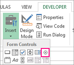
Once the sphere appears to be like in the cell, replica it, highlight the cells you also favor it to appear in, after which paste it.

17. Hyperlink a cell to a internet based attach.

For fogeys that’re the use of your sheet to computer screen social media or internet attach metrics, it will also be worthy to occupy a reference column with the links every row is monitoring. For fogeys that add a URL straight into Excel, it could possibly perhaps possibly automatically be clickable. However, whenever you would possibly want to hyperlink words, equivalent to a page title or the headline of a put up you’re monitoring, here’s how.

Spotlight the words you’d like to must hyperlink, then press Shift K. From there a field will pop up allowing you to predicament the hyperlink URL. Reproduction and paste the URL into this field and hit or click on Enter.

If basically the vital shortcut is no longer genuinely working for any cause, you must possibly perhaps possibly possibly also also enact this manually by highlighting the cell and clicking Insert > Hyperlink.

18. Add drop-down menus.

Veritably, you can be succesful of be the use of your spreadsheet to computer screen processes or diversified qualitative things. In choice to writing words into your sheet repetitively, equivalent to “Yes”, “No”, “Customer Stage”, “Sales Lead”, or “Prospect”, you must possibly perhaps possibly possibly also use dropdown menus to speedily mark descriptive things about your contacts or irrespective of you’re monitoring.

Here is easy methods on how so as to add drop-downs to your cells.

Spotlight the cells you’d like to occupy the drop-downs to be in, then click on the Files menu in the high navigation and press Validation.

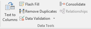
From there, you can be succesful of gaze a Files Validation Settings field commence. Leer at the Allow recommendations, then click on Lists and employ Fall-down Record. Test the In-Cell dropdown button, then press OK.

A form of Excel Succor Resources

• The correct arrangement to Scheme a Chart or Graph in Excel [With Video Tutorial]
• Set up Tips to Originate Stunning Excel Charts and Graphs
• Totally Free Microsoft Excel Templates That Scheme Marketing More uncomplicated
• The correct arrangement to Learn Excel On-line: Free and Paid Resources for Excel Practicing

Use Excel to Automate Processes in Your Crew

Even whenever you’re no longer an accountant, you must possibly perhaps possibly possibly also restful use Excel to automate tasks and processes in your crew. With the methods and tricks we shared in this put up, you’ll make sure to make use of Excel to its fullest extent and earn basically the most out of the machine to develop your industry.

Editor’s Demonstrate: This put up became as soon as at the initiating revealed in August 2017 nonetheless has been up previously for comprehensiveness.

Initially revealed Jul 1, 2021 7: 00: 00 AM, up previously July 01 2021