How to Use VLOOKUP Function in Microsoft Excel [+ Video Tutorial]

Coordinating a huge amount of information in Microsoft Excel is a time-ingesting headache. That headache can even be made even worse if you desire to examine info across more than one spreadsheets. The final ingredient you desire to achieve is manually switch cells the usage of reproduction and paste. Fortunately, you don’t desire to. The VLOOKUP function may perhaps well help you to automate this assignment and keep you a complete bunch time.

I know, “VLOOKUP function” sounds love the geekiest, most sophisticated ingredient ever. But by the time you produce reading this article, you may perhaps well marvel how you ever survived in Excel with out it.

Microsoft Excel’s VLOOKUP function is more uncomplicated to make exhaust of than you mediate. What’s more, it is incredibly great, and is surely something you desire to beget to your arsenal of analytical weapons.What does VLOOKUP attain, precisely? Right here is the easy explanation: The VLOOKUP function searches for a impart worth to your info, and as soon as it identifies that worth, it would secure — and display — some diversified fragment of information that is expounded to that worth.

How does VLOOKUP work?

VLOOKUP stands for “vertical search for.” In Excel, this implies the act of taking a sight up info vertically across a spreadsheet, the usage of the spreadsheet’s columns — and a selected identifier inside of these columns — as the premise of your search. Even as you survey up your info, it’ll also simply tranquil be listed vertically wherever that info is found.

The procedure frequently searches to the finest.

When conducting a VLOOKUP in Excel, you are in actuality shopping for imprint new info in a selected spreadsheet that is expounded to dilapidated info to your recent one. When VLOOKUP runs this search, it frequently appears for the new info to the appropriate of your recent info.

As an illustration, if one spreadsheet has a vertical checklist of names, and one other spreadsheet has an unorganized checklist of these names and their electronic mail addresses, you may perhaps well be ready to exhaust VLOOKUP to retrieve these electronic mail addresses in the present that you just can beget them to your first spreadsheet. These electronic mail addresses can even simply tranquil be listed in the column to the finest of the names in the 2nd spreadsheet, or Excel can even simply now not be ready to search out them. (Lunge figure … )

The procedure wants a selected identifier to retrieve info.

The secret to how VLOOKUP works? Unfamiliar identifiers.

A diversified identifier is a fragment of information that both of your info sources piece, and — as its name implies — it is bizarre (i.e. the identifier is totally linked to 1 file to your database). Unfamiliar identifiers consist of product codes, inventory-retaining devices (SKUs), and buyer contacts.

Alright, enough explanation: let’s perceive one other instance of the VLOOKUP in stride!

VLOOKUP Example

In the video underneath, we are going to display an instance in stride, the usage of the VLOOKUP function to examine electronic mail addresses (from a 2nd info source) to their corresponding info in a separate sheet. 

Creator’s expose: There are many various variations of Excel, so what you perceive in the video above can even simply now not frequently match up precisely with what you may perhaps well perceive to your model. That is why we attend you to notice along with the written instructions underneath.

For your reference, right here’s what a VLOOKUP function appears love:

VLOOKUP(lookup_value , table_array , col_index_num , range_lookup)

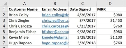
In the steps underneath, we are going to keep the finest worth to each of these procedure, the usage of buyer names as our bizarre identifier to search out the MRR of every buyer.

1. Identify a column of cells you’d love to beget with new info.

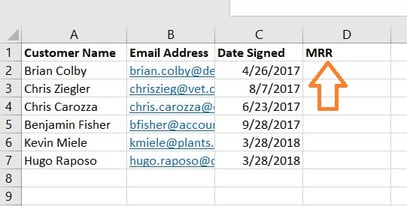
Endure in ideas, you take a sight to retrieve info from one other sheet and deposit it into this one. With that in ideas, imprint a column subsequent to the cells you wish more info on with a simply title in the tip cell, equivalent to “MRR,” for month-to-month recurring income. This new column is where the records you are fetching will poke.

2. Make a choice ‘Characteristic’ (Fx) > VLOOKUP and insert this procedure into your highlighted cell.

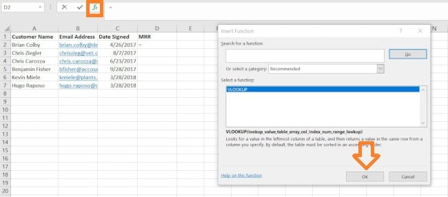
To the left of the text bar above your spreadsheet, you may perhaps well perceive a miniature function icon that appears love a script: Fx. Click on on the predominant empty cell underneath your column title and then click this function icon. A box titled Arrangement Builder or Insert Characteristic will seem to the finest of your display disguise (looking on which model of Excel that you just can beget).

Look for and prefer out “VLOOKUP” from the checklist of alternate choices included in the Arrangement Builder. Then, prefer out OK or Insert Characteristic to birth constructing your VLOOKUP. The cell you presently beget highlighted to your spreadsheet can even simply tranquil now survey love this: “=VLOOKUP()“

You may perhaps well perhaps also enter this procedure accurate into a name manually by coming into the daring text above precisely into your desired cell.

With the =VLOOKUP text entered into your first cell, it be time to beget the procedure with four diversified criteria. These criteria may perhaps well help Excel narrow down precisely where the records you wish is found and what to gaze.

3. Enter the search for worth for which you desire to retrieve new info.

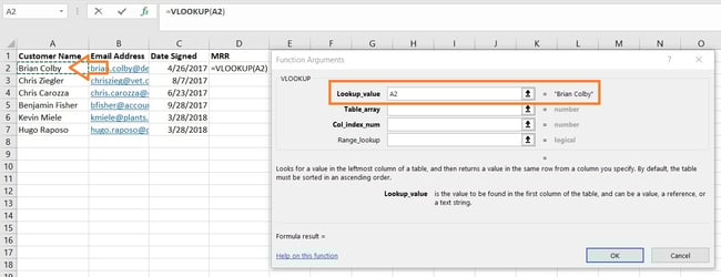
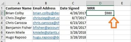
The first criteria is your search for worth — that is the worth of your spreadsheet that has info linked to it, which you wish Excel to search out and return for you. To enter it, click on the cell that carries a imprint you are seeking to search out a match for. In our instance, confirmed above, it be in cell A2. You’ll birth migrating your new info into D2, since this cell represents the MRR of the shopper name listed in A2.

Hold in ideas your search for worth can even be the leisure: text, numbers, net net page links, you name it. As long as the worth you take a sight up matches the worth in the referring spreadsheet — which we are going to advise about that in the following step — this function will return the records you wish.

4. Enter the desk array of the spreadsheet where your desired info is found.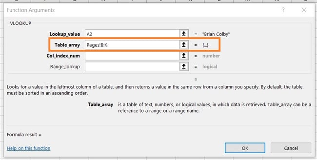

Subsequent to the “desk array” discipline, enter the vary of cells you’d love to poke trying and the sheet where these cells are positioned, the usage of the format confirmed in the screenshot above. The entry above potential the records we’re shopping for is in a spreadsheet titled “Pages” and can even be found anywhere between column B and column K.

The sheet where your info is found can even simply tranquil be inside of your recent Excel file. This implies your info can both be in a selected desk of cells somewhere to your recent spreadsheet, or in a selected spreadsheet linked on the underside of your workbook, as confirmed underneath.

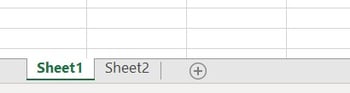
As an instance, in case your info is found in “Sheet2” between cells C7 and L18, your desk array entry will be “Sheet2!C7:L18.”

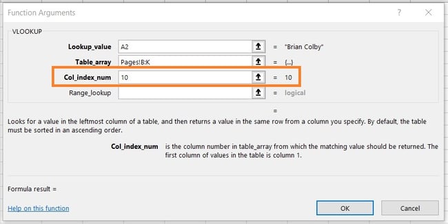
5. Enter the column series of the records you wish Excel to return.

Beneath the desk array discipline, you may perhaps well enter the “column index number” of the desk array you are shopping through. As an instance, in case you are focusing on columns B through K (notated “B:K” when entered in the “desk array” discipline), however the impart values you wish are in column K, you may perhaps well enter “10” in the “column index number” discipline, since column K is the 10th column from the left.

6. Enter your vary search for to search out an valid or approximate match of your search for worth.

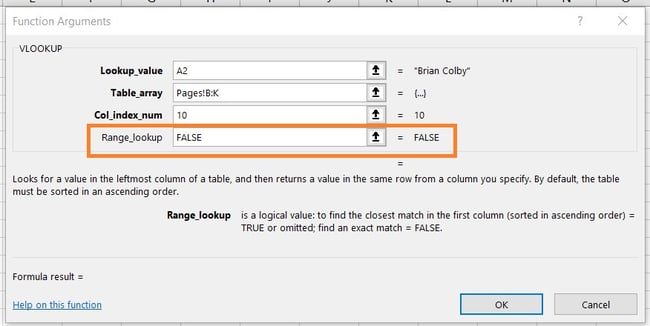
In situations love ours, which concerns month-to-month income, you desire to search out valid matches from the desk you are shopping through. To attain this, enter “FALSE” in the “vary search for” discipline. This tells Excel you desire to search out completely the impart income linked to each gross sales contact.

To acknowledge to your burning query: Yes, you may perhaps well be ready to enable Excel to gaze an approximate match as a change of an valid match. To attain so, simply enter TRUE as a change of FALSE in the fourth discipline confirmed above.

When VLOOKUP is decided for an approximate match, it be shopping for info that most carefully resembles your search for worth, in dwelling of information that is such as that worth. Even as you take a sight up info linked to a list of net net page links, as an instance, and a few of your links beget “https://” before the whole lot, it may perhaps well perhaps behoove you to search out an approximate match factual in case there are links that attain now not beget this “https://” imprint. This methodology, the leisure of the hyperlink can match with out this initial text imprint inflicting your VLOOKUP procedure to return an error if Excel can now not secure it.

7. Click on ‘Completed’ (or ‘Enter’) and beget your new column.

In present to formally elevate in the values you wish into your new column from Step 1, click “Completed” (or “Enter,” relying to your model of Excel) after filling the “vary search for” discipline. This can even simply populate your first cell. You may perhaps well perhaps clutch this chance to survey in the diversified spreadsheet to ensure this turned into the simply worth.

If that’s the case, populate the leisure of the new column with each subsequent worth by clicking the predominant filled cell, then clicking the little sq. that seems to be on the underside-appropriate corner of this cell. Completed! Your complete values can even simply tranquil seem.

VLOOKUP No longer Working?

When that you just can beget followed the above steps and your VLOOKUP is tranquil now not working, this may perhaps well both be a scheme back along with your:

• Syntax (i.e. how that you just can beget structured the procedure)
• Values (i.e. whether or now not the records it be taking a sight up is honest and formatted as it’ll be)

Troubleshooting VLOOKUP Syntax

Commence with taking a sight on the VLOOKUP procedure that you just may perhaps beget written in the designated cell.

• Is it relating to the finest search for worth for its key identifier?
• Does it specify the simply desk array vary for the values it wants to retrieve
• Does it specify the simply sheet for the vary?
• Is that sheet spelled as it’ll be?
• Is it the usage of the simply syntax to discuss with the sheet? (e.g. Pages!B:K or ‘Sheet 1’!B:K)
• Has the simply column number been specified? (e.g. A is 1, B is 2, and so on)
• Is Appropriate or Deceptive the simply route for how your sheet is decided up?

Troubleshooting VLOOKUP Values

If the syntax is now not the discipline, how you would also simply beget a scheme back with the values you are seeking to bag themselves. This most frequently manifests as an #N/A error where the VLOOKUP can’t secure a referenced worth.

• Are the values formatted vertically and from appropriate to left?
• Manufacture the values match how you discuss with them?

As an instance, in case you take a sight up URL info, each URL can even simply tranquil be a row with its corresponding info to the left of it in the same row. When that you just can beget the URLs as column headers with the records intelligent vertically, the VLOOKUP will now not work.

Maintaining with this instance, the URLs need to examine in format in both sheets. When that you just can beget one sheet at the side of the “https://” in the worth whereas the diversified sheet omits the “https://”, the VLOOKUP will now not be ready to examine the values.

VLOOKUPs as a Extremely wonderful Marketing and marketing Tool

Entrepreneurs wish to analyze info from a vary of sources to bag a complete image of lead generation (and more). Microsoft Excel is the finest instrument to achieve this precisely and at scale, namely with the VLOOKUP function.

Editor’s expose: This post turned into before the whole lot printed in March 2019 and has been updated for comprehensiveness.

Before the whole lot printed Jul 14, 2021 1: 15: 00 PM, updated July 14 2021